
Earthquake Science and the San Andreas Fault for Geology Exams
Learn how to study earthquake science and the San Andreas Fault for your geology exam using a concept-first approach that connects stress, faulting, seismic waves, and measurement through the San Andreas Fault as a real-world case study.
Updated:
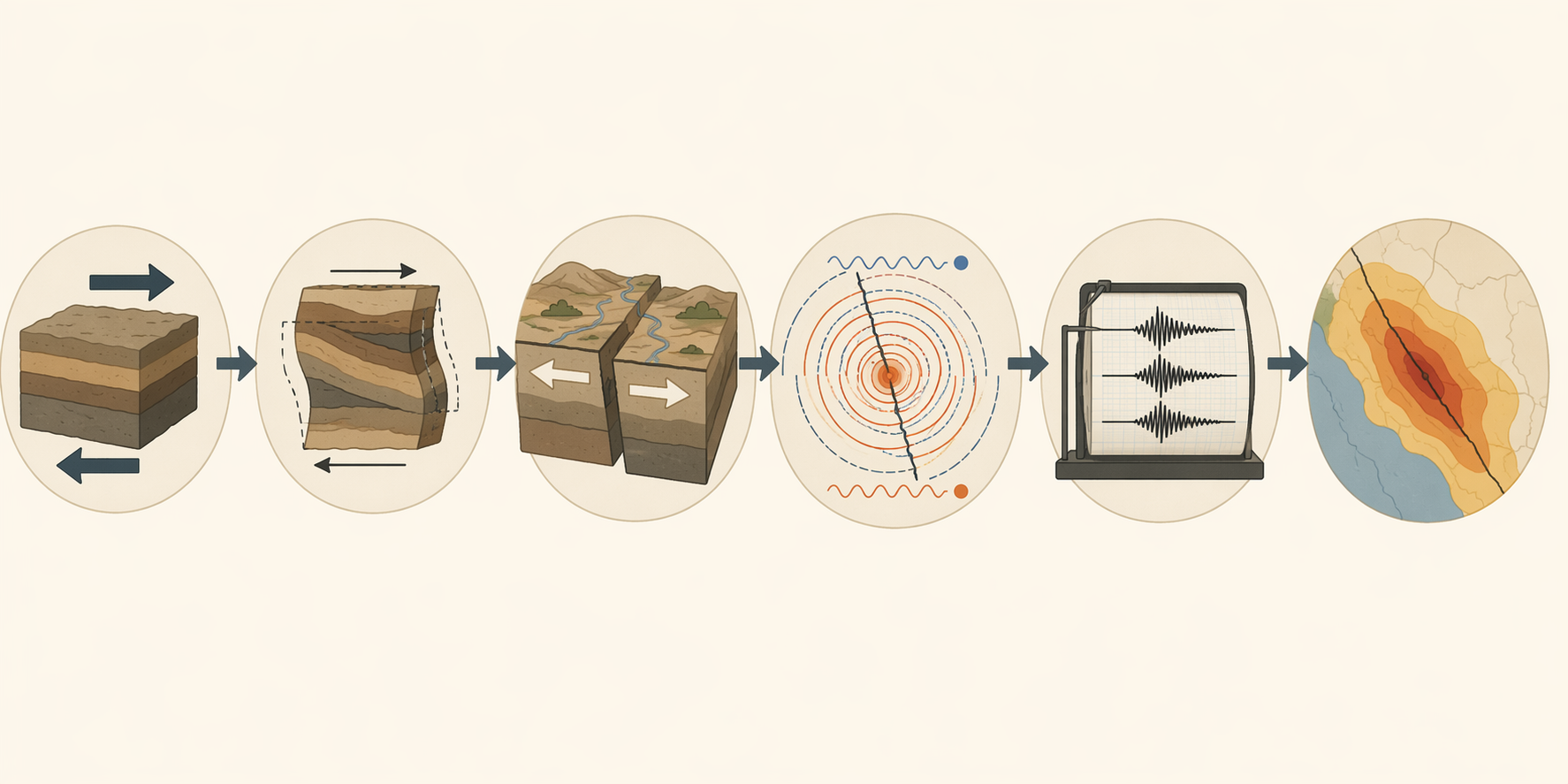
If your geology exam covers earthquakes and the San Andreas Fault, do not start by memorizing a loose pile of terms. Start with the chain your instructor is probably testing: stress acts on rock, rock deforms as strain builds, a fault slips when the rock fails, seismic waves carry the released energy, seismographs record those waves, and geologists use the records plus fault history to estimate hazard.
The San Andreas Fault is useful because one real example can carry that whole chain. It is a right-lateral strike-slip transform boundary between the Pacific Plate and the North American Plate, extending roughly 1,200 to 1,300 km through California, with commonly cited slip-rate estimates in the range of about 20 to 35 mm per year.[1][2] Those numbers matter less as trivia than as labels for a system: plates move, shear stress accumulates, fault segments either creep or lock, and earthquakes happen where stored elastic strain is suddenly released.
Study the Unit as One Chain
A good exam answer usually does not stop at naming a feature. If the prompt shows arrows pulling rock apart, you identify tension, then a normal fault, then a likely divergent setting. If the arrows push together, you identify compression, then a reverse or thrust fault, then a convergent setting. If the arrows slide past one another, you identify shear, then a strike-slip fault, then a transform setting.[3]
| Start with | Then connect it to | Exam move |
|---|---|---|
| Stress | Tension, compression, or shear | Draw arrows before naming the fault |
| Fault motion | Normal, reverse/thrust, or strike-slip | Show which block moves and why |
| San Andreas example | Right-lateral strike-slip transform motion | Connect lateral motion to the Pacific-North American plate boundary |
| Elastic rebound | Stored strain released suddenly | Explain why a fault can be quiet before a large earthquake |
| Seismic waves | P, S, Love, and Rayleigh waves | Use arrivals and wave behavior, not just names |
| Measurement | S-P interval, epicenter, magnitude, intensity | Separate location, energy, and observed shaking |
| Hazard | Past ruptures, recurrence, probabilities, local conditions | Discuss risk without pretending to predict the exact next earthquake |
That table is not a replacement for studying. It is the order of operations. When a diagram or word problem appears, work left to right through the chain instead of grabbing the first vocabulary word that looks familiar.
Turn Stress into Fault Types Before You Memorize Names
Fault names make more sense after the stress arrows are in place. Tension stretches crust and commonly produces normal faults. Compression shortens crust and commonly produces reverse faults or low-angle thrust faults. Shear moves rock masses sideways past one another and produces strike-slip faults.[3][4]
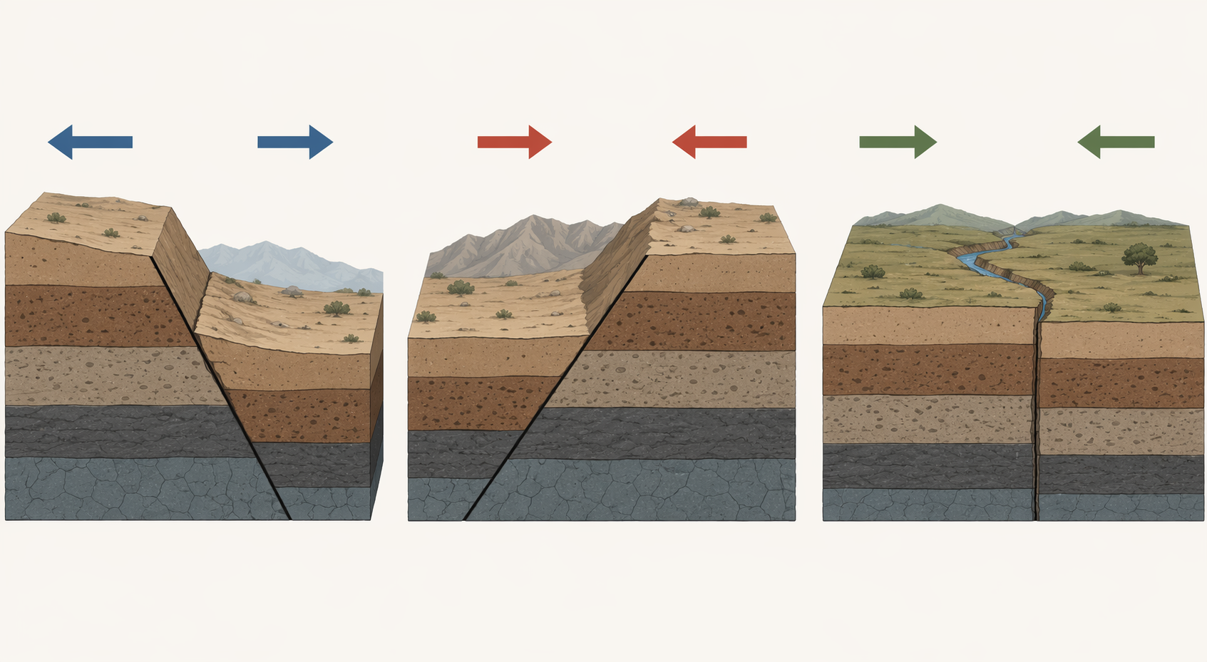
On a lab sheet, draw the arrows first. For a normal fault, draw the crust being pulled apart and the hanging wall moving down relative to the footwall. For a reverse fault, draw compression and the hanging wall moving up. For a strike-slip fault, stop looking for a hanging wall and footwall as the main clue; the important motion is horizontal.
The San Andreas Fault belongs in that third category. It is a transform fault, and the relative motion is right-lateral strike-slip: if you stand on one side of the fault and look across it, the opposite side appears to move to your right.[1][2] That sentence is worth practicing aloud because students often know the phrase “right-lateral” but freeze when asked to identify it from a map or offset stream.
A quick drawing test for right-lateral motion
Draw a vertical fault line on scratch paper. Put one arrow upward on the left side and one arrow downward on the right side. Now imagine standing on either block and looking across the fault. The far block moves to your right. That is right-lateral motion. The San Andreas is the example you can attach to that sketch.
Elastic Rebound Is the Mechanism, Not a Historical Footnote
Elastic rebound theory is where the earthquake unit starts behaving like a system. Rocks near a fault can bend elastically as tectonic stress continues. If the fault is locked, strain accumulates. When the strength of the rock or frictional resistance is exceeded, the fault slips, the deformed rocks rebound toward a less strained shape, and seismic energy is released.[5]
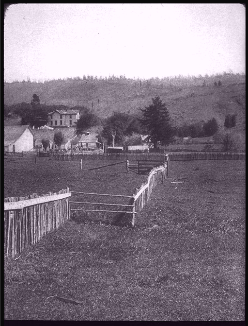
This is why the 1906 San Francisco earthquake belongs in your notes. After that earthquake, H. F. Reid used observations of displaced features, including offsets across the San Andreas Fault, to develop elastic rebound theory.[5] The point is not merely that a fence moved. The offset is visible evidence that strain had accumulated before rupture and was released during fault slip.
For exam purposes, the clean version is: tectonic stress slowly loads the crust; locked rock near the fault stores elastic strain; rupture releases that strain as sudden slip; seismic waves carry energy away. If you can explain that sequence, you can answer more than one kind of question: a diagram of bent fence lines, a short-answer prompt about why earthquakes recur, or a multiple-choice item asking what elastic rebound actually describes.
Locked Segments and Creeping Segments Explain Why One Fault Behaves Unevenly
A beginner mistake is to treat the whole San Andreas as if it behaves the same way everywhere. It does not. The fault is commonly divided into northern, central, and southern sections. The northern section ruptured in the 1906 earthquake, with rupture extending for roughly 430 km. The central section includes a creeping portion often described as about 130 km long, where aseismic creep releases strain gradually at about 3 cm per year. The southern section is often discussed as locked, with recurrence estimates near 140 to 160 years and the potential for very large earthquakes in some scenarios.[1]
That creeping central section is not an exception to ignore. It is the nuance that improves an exam answer. A fault can accommodate plate motion through sudden earthquakes, slow creep, or some combination depending on the segment. “Fault” does not automatically mean “large earthquake at every point.” It means a fracture or fracture zone along which rock masses have moved, and the style of movement matters.[6]
The same distinction helps with historical examples. The 1857 Fort Tejon earthquake is the major southern San Andreas rupture commonly cited at about magnitude 7.9. The 1906 San Francisco earthquake, usually given as about magnitude 7.8 to 7.9, anchors the northern rupture and elastic rebound story. The 1989 Loma Prieta earthquake, at magnitude 6.9, is a familiar California earthquake reference, but for an introductory exam it is usually less central than 1906 for explaining mechanism.[1]
Follow the Released Energy into Seismic Waves
Once rupture happens, the next exam question often moves from fault mechanics to wave behavior. The earthquake focus, or hypocenter, is the place inside Earth where rupture begins. The epicenter is the point on Earth’s surface directly above it.[6] Keep those two labels separate on diagrams: focus underground, epicenter at the surface.
P-waves arrive first because they are the fastest seismic body waves. They are compressional waves and can travel through solids, liquids, and gases. S-waves arrive later; they are shear waves and travel through solids but not liquids. Surface waves, including Love and Rayleigh waves, travel along Earth’s surface and are generally slower than body waves, but they often produce the strongest damaging shaking near the surface.[3][6]
| Wave type | Motion | Where it travels | Exam clue |
|---|---|---|---|
| P-wave | Compressional push-pull | Solids, liquids, and gases | First arrival on a seismogram |
| S-wave | Shear motion | Solids only | Second body-wave arrival |
| Love wave | Horizontal surface motion | Along the surface | Surface wave associated with damaging shaking |
| Rayleigh wave | Rolling surface motion | Along the surface | Surface wave associated with damaging shaking |
On a seismogram worksheet, do not label the biggest wiggle as the P-wave just because it catches your eye. Find the first arrival. Then find the S-wave arrival. The time gap between them is the S-P interval, and that gap grows as distance from the earthquake increases.[4]
Use S-P Intervals to Locate the Epicenter
Epicenter problems usually look procedural, but they are still concept questions. P-waves travel faster than S-waves, so the farther a seismic station is from the earthquake, the larger the arrival-time difference becomes. A travel-time graph converts that S-P interval into distance from the station.[4]
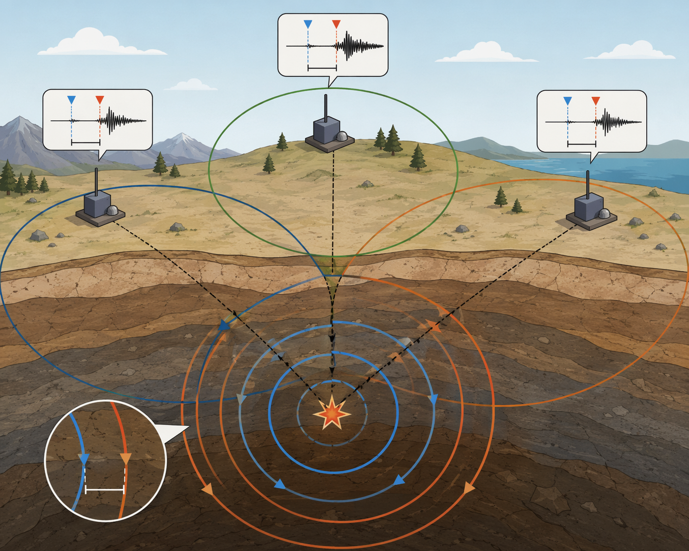
The station distance alone does not give direction. It gives a circle around the station. With three stations, three distance circles intersect near the epicenter.[4] If your circles do not meet perfectly, your instructor may expect the best common intersection area rather than a mathematically perfect point, especially on a hand-drawn lab map.
- Mark the P-wave arrival on each seismogram.
- Mark the S-wave arrival on each seismogram.
- Subtract to find the S-P interval.
- Use the travel-time curve to convert the interval into distance.
- Draw one circle around each station using that distance.
- Identify the epicenter where the circles intersect or cluster.
This is also where the San Andreas can stay in the background without taking over. If an earthquake occurs on a California strike-slip fault, seismograms at different stations will still show P and S arrivals. The method for locating the epicenter does not change because the named fault is famous.
Magnitude Is Not the Same as Intensity
Magnitude estimates the size of the earthquake at its source. Intensity describes the shaking effects at a particular location. That distinction is easy to say and easy to lose under exam pressure. One earthquake has one magnitude value in the usual reporting sense, but it can produce many intensity values because shaking varies with distance, ground conditions, building type, and other local factors.[4][6]
The common numerical trap is the difference between amplitude and energy. For each whole-number increase in magnitude, measured wave amplitude increases by a factor of 10, while energy release increases by about 32 times.[4] So a magnitude 7 earthquake does not release ten times the energy of a magnitude 6 earthquake; the exam answer is about 32 times the energy.
Moment magnitude, written Mw, is now preferred for large earthquakes because it is based on seismic moment and better represents very large events than the older Richter scale in many contexts.[4] The Modified Mercalli Intensity scale, by contrast, is qualitative: it describes observed effects of shaking at specific places.[6] If a question asks what people felt and what damage occurred in different towns, it is asking about intensity, not source magnitude.
Use the San Andreas for Hazard Reasoning, Not Prediction
Hazard questions ask how geologists reason from faults, past earthquakes, and ground conditions toward future risk. They do not ask you to name the exact day of the next earthquake. For the San Andreas Fault, that reasoning includes plate-boundary motion, locked and creeping behavior, past ruptures, and the fact that not all Pacific-North American motion is carried by the San Andreas itself. One summary source describes the San Andreas as accommodating about 75% of relative Pacific-North American plate motion, with the remaining motion distributed across zones such as the Eastern California Shear Zone and Walker Lane.[1]
Paleoseismology is the bridge between “we know earthquakes happened” and “we can estimate recurrence.” Geologists dig trenches across active faults, identify disturbed sediment layers, and use methods such as radiocarbon dating and dendrochronology to estimate the timing of prehistoric earthquakes.[7] Intro-level exams usually do not require you to run the dating method. They want you to know why a trench can reveal earthquakes older than written records.
Those records feed probabilistic hazard models. UCERF3, the third Uniform California Earthquake Rupture Forecast, estimated a 7% probability of a magnitude 8 or larger earthquake in California over 30 years.[8] Treat that as probability, not prophecy. It is a model-based estimate over a time window, not a schedule.
Recent research can enrich this part of your notes if your class discusses current events. A University of Hawaiʻi news release in June 2026 reported that Burkhard and coauthors found tectonic stress along the southern San Andreas and San Jacinto fault system at the highest level in 1,000 years, with Cajon Pass described as a possible “earthquake gate” for a linked rupture scenario.[9] The related journal article focuses on stress accumulation and rupture-path implications in the Cajon Pass region.[10] That is useful context, especially in Q3 2026, but it should not replace the basic exam chain: stress, strain, rupture, waves, measurement, hazard.
What to Be Able to Do Before the Exam
A strong study session ends with performance, not rereading. Close the textbook and explain the full earthquake chain aloud from stress to hazard. If you cannot move smoothly from one link to the next, that is the gap to fix.
- Sketch normal, reverse, and strike-slip faults from stress arrows, then label the motion.
- Identify the San Andreas Fault as a right-lateral strike-slip transform boundary between the Pacific and North American plates.
- Explain elastic rebound using locked fault behavior, accumulated strain, sudden slip, and the 1906 San Francisco earthquake example.
- Distinguish P-waves, S-waves, Love waves, and Rayleigh waves by arrival order, motion, travel medium, and likely surface effects.
- Solve or describe an S-P interval triangulation problem using three seismic stations.
- Separate magnitude from intensity, and remember that one magnitude unit means 10 times amplitude but about 32 times energy.
- Discuss hazard using recurrence, paleoseismology, locked versus creeping segments, and probability without claiming exact prediction.
That is the reason the San Andreas Fault is such a good study example. It is not just a famous California fault to memorize. It lets you practice the connected reasoning your exam is likely to reward: stress creates strain, strain is released by fault slip, rupture sends out waves, instruments record arrivals, and geologists use those records and the fault’s history to estimate hazard.
References
- “San Andreas Fault” — Wikipedia
- “The San Andreas Fault: Facts about the crack in California's crust” — Live Science
- “9 Crustal Deformation and Earthquakes” — OpenGeology Textbook
- “Earthquakes & Earth's Interior” — Tulane University
- “Elastic Rebound” — U.S. Geological Survey
- “The Science of Earthquakes” — U.S. Geological Survey
- “Introduction to Paleoseismology” — U.S. Geological Survey
- “Back to the Future on the San Andreas Fault” — U.S. Geological Survey
- “San Andreas fault reaches highest stress level in 1,000 years” — University of Hawaiʻi System News, June 10, 2026
- “Cajon Pass and the Southern San Andreas Fault System” — Burkhard et al., JGR: Solid Earth, 2025
Comments
Join the discussion with an anonymous comment.