
Method
How scientists study flash flood risk in the Tahoe Basin
Scientists use four distinct research methods to assess flash flood risk in the Lake Tahoe Basin: hydrologic simulation, extreme-storm scenario modeling, indicator-based vulnerability frameworks, and machine learning prediction. This article walks through each method and shows how their combined findings point to a near-doubling of flood risk.
Evidence panel
- Evidence level
- High
- Primary citation
- Desert Research Institute (2023). More Heatwaves and Vanishing Snow: The Lake Tahoe Basin's Future on a Warming Planet.
Studying flash flood risk in the Lake Tahoe Basin starts with a physical inconvenience: the basin is not a flat test plot. Water falls as rain, snow, or rain-on-snow across steep Sierra Nevada terrain, moves through small tributaries with different slopes and soils, collects around communities and roads, and responds strongly to atmospheric-river storms. UC Davis Tahoe Environmental Research Center director Geoffrey Schladow has described one atmospheric-river mechanism in concrete terms: a single event could raise Lake Tahoe’s water level by 1 foot per day, while peak streamflows could potentially triple.[1]
That is why a serious study of Tahoe flash flood risk cannot be only a rainfall study, only a damage study, or only a map. The research problem has layers. One method has to ask how climate inputs change runoff and streamflow. Another has to ask what happens if an extreme storm sequence parks over the region. A third has to ask which places and structures are more vulnerable once water arrives. A fourth can look for predictive patterns in long meteorological records. The useful lesson is not that more methods automatically mean better science; it is that each method is built to see a different part of the same risk system.
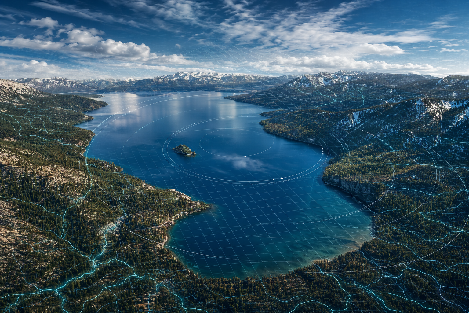
The physical model: dividing the basin finely enough to ask local questions
The most instructive starting point is the Desert Research Institute’s Lake Tahoe Basin hydrologic simulation. The study used the Precipitation-Runoff Modeling System, or PRMS, to represent how precipitation, temperature, snowpack, evapotranspiration, soil storage, and streamflow interact across the basin. The model divided the basin into 60 subbasins and drove future projections with more than 8 global climate models under two emissions pathways, RCP4.5 and RCP8.5.[2]
For students learning research design, the eye-catching part is the grid. The DRI work moved from a previous spatial resolution of 14 square miles to 1/29 square mile.[2] That is not just a prettier map. A 14-square-mile cell can blur together terrain, tributaries, and neighborhoods that behave differently during a warm storm. A 1/29-square-mile unit lets researchers ask more local questions: which subbasin responds more sharply, where snow loss changes the timing of runoff, and how a smaller stream network might behave under a warmer storm regime.
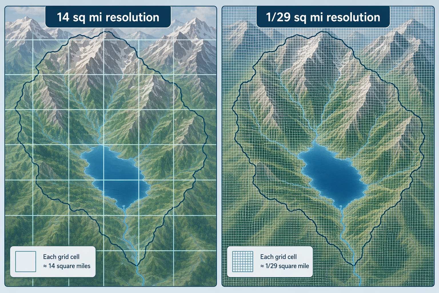
The distinction matters because basin-scale averages can hide the very places where flash flood risk becomes operational. A watershed planner does not only need to know that the basin is getting warmer. She needs to know which tributaries may see larger peaks, whether more winter precipitation arrives as rain rather than snow, and whether streamflow changes concentrate in particular drainage areas. Finer spatial design gives the model a chance to represent those differences.
But finer resolution is not the same thing as truth. A small grid cell can still inherit poor climate inputs, weak calibration, missing land-surface processes, or uncertain assumptions about future emissions. Resolution changes the scale of possible questions; it does not remove uncertainty. This is a useful discipline to keep in mind because model graphics often imply a confidence that the underlying data may not fully deserve.
The DRI projections are still important because the model design is tied to a clear physical question: what happens to Tahoe hydrology as the basin warms? The study projected 4–9°F of warming and, across six monitored streams, a 65–117% increase in the magnitude of 20-year floods.[2] That latter number is not a count of floods; it describes how large a flood of a given return category could become under the modeled future conditions. In plain terms, the same class of event can carry more water.
The mechanism is not mysterious. Warmer conditions can reduce snow storage, shift precipitation toward rain, and accelerate runoff timing. In a mountain basin, snowpack often acts as temporary storage. When more storm water runs off quickly instead of waiting as snow, peak flows can rise. That is exactly the kind of physical pathway a distributed hydrologic model is meant to test.
One limitation deserves more than a footnote: the DRI projections deliberately excluded post-wildfire landscape change.[2] That exclusion makes the model cleaner, but not complete. Burned landscapes can change infiltration, erosion, vegetation cover, and runoff response. For a student building a proposal, this is a good example of a defensible modeling boundary that also narrows the conclusion. The model can speak to climate-driven hydrologic change as represented in its design; it should not be stretched into a full post-fire flood-risk estimate.
From projection to stress test: what ARkStorm adds
Hydrologic projections ask how the basin’s flood regime may change under future climate conditions. The ARkStorm work asks a different question: what if a severe atmospheric-river sequence hit California and the Sierra Nevada as a long-duration emergency? The ARkStorm scenario is built around a hypothetical 23-day storm sequence and has been used to estimate $725 billion in economic damage for California alone, a figure described as more than triple Hurricane Katrina.[3]
That number is vivid, but it should be handled carefully. ARkStorm is not a forecast that says California, Tahoe, or the Sierra Front will experience that exact damage on a particular schedule. It is also not probability-weighted in the way a return-period estimate or probabilistic risk model might be. Its value is as a stress test: a scenario that lets researchers, emergency managers, and infrastructure planners examine what systems might fail, which corridors could be isolated, and what cascading consequences might follow during an extreme atmospheric-river sequence.
That difference between projection and scenario is not semantic. A climate-driven hydrologic model can estimate how stream behavior changes across modeled futures. A scenario model can push emergency systems into an extreme but plausible sequence and expose planning weaknesses. One estimates changing conditions; the other rehearses consequences under a constructed event. Confusing the two is how a stress-test number gets misread as a prediction.
The vulnerability framework: when the question shifts from water to harm
A flood hazard map does not automatically tell us who or what is most likely to suffer damage. Two buildings can sit near the same drainage pathway and face different consequences because of foundation type, age, floor height, material, or value. This is where indicator-based vulnerability frameworks become useful. They do not simulate every drop of water. They assemble measurable factors into an index that ranks hazard and vulnerability across space.
Zhen et al. built that kind of framework by separating the physical hazard side from the built-environment vulnerability side. Their Flash Flood Hazard Index used six indicators: elevation, slope, drainage density, soil type, land use, and rainfall intensity. Their Vulnerability Index used five building indicators: building material, structure age, foundation type, floor height, and building value.[4]
| Index | What it tries to measure | Indicators used |
|---|---|---|
| Flash Flood Hazard Index | Where flash flooding is physically more likely or more intense | Elevation; slope; drainage density; soil type; land use; rainfall intensity |
| Vulnerability Index | Which buildings are more likely to suffer harm if exposed | Building material; structure age; foundation type; floor height; building value |
The delicate part of this method is weighting. If slope receives too much weight, the index may overemphasize steep terrain. If building value dominates, the index may privilege expensive property over physical fragility. If rainfall intensity is underweighted, the hazard score can become a terrain map with weather pasted on top. Indicator frameworks look simple only after the hardest judgment has already been made: deciding how much each variable should count.
Zhen et al. addressed that problem with a three-part weighting strategy. First, they used the Analytic Hierarchy Process, drawing on judgments from 30 expert panelists. Second, they trained a Random Forest model on 117 post-disaster buildings, allowing observed damage patterns to inform the weights. Third, they used Game Theory through Shapley values to reconcile the AHP and Random Forest weights.[4]
That architecture is worth slowing down over. AHP brings in expert reasoning: people with domain knowledge compare the relative importance of indicators. Random Forest brings in empirical learning from damaged buildings: the model looks for which variables best separate observed outcomes. Shapley values then provide a way to arbitrate between the expert-derived and data-derived views. The framework is not simply asking experts to vote, nor is it pretending that 117 buildings can settle the whole question by themselves.[4]
This is a different research logic from PRMS. The hydrologic simulation is strongest when the question is how climate and basin processes change runoff and streamflow. The vulnerability framework is strongest when the question is how physical exposure and building characteristics translate into likely damage. It also carries a different kind of uncertainty. The result depends on indicator selection, data quality, weighting rules, and whether the post-disaster training sample represents the range of buildings and flood conditions that future events may produce.
Machine learning as a pattern-finding layer
Machine learning enters the Tahoe flash flood risk problem from another angle: prediction from historical meteorological patterns. Devi et al. used XGBoost with more than 50 years of meteorological records to forecast flood levels, reporting R² = 0.945 and MAE = 0.514 mm. The model was paired with HEC-RAS 2D hydraulic modeling to produce spatial inundation mapping, and feature-importance analysis was used to identify which meteorological variables most strongly drove the predictions.[5]
The useful contribution here is not that XGBoost is fashionable. It is that a machine-learning model can search a long meteorological record for nonlinear relationships that may be difficult to specify manually. Feature importance can also help students see which inputs the model is leaning on. In a flood-risk assessment, that can make machine learning a screening or forecasting layer rather than a replacement for hydrologic reasoning.
The reported R² is strong, but high in-sample or study-specific performance does not by itself prove broad generalizability. If a model depends heavily on a few variables, performs well under the distribution represented in its training data, or is calibrated to a particular basin context, it may weaken when moved to a different watershed or to future conditions outside the historical range. That is not a criticism unique to XGBoost; it is the ordinary caution required when a predictive model is asked to travel beyond the data environment that trained it.
Why the near-doubling signal is more persuasive across methods
The strongest case for increased Tahoe flash flood risk does not rest on a single dramatic number. It comes from convergence. The DRI hydrologic work projects substantially larger future flood magnitudes, including a 65–117% increase in 20-year floods across six monitored streams.[2] Separate atmospheric-river damage research by Corringham et al. projected annual damages across the Western United States rising from about $1 billion to $2.3–3.2 billion, while holding present-day exposure and vulnerability constant.[6]
That last condition matters. Holding exposure and vulnerability constant means the Corringham et al. estimate is not a full prediction of what future damages will actually be. Development patterns, building codes, insurance penetration, mitigation work, and population change could push real damages higher or lower. The study is better read as evidence of how climate-related atmospheric-river damages may change under a controlled exposure assumption, not as a complete social forecast.[6]
The methods do not all measure the same object. PRMS estimates physical hydrologic response. GEV-style stream analysis summarizes changes in flood magnitude for monitored streams. ARkStorm stress-tests an extreme atmospheric-river sequence. Indicator frameworks organize hazard and vulnerability variables. Machine learning searches historical meteorological data for predictive structure. Their weaknesses also differ: calibration limits, scenario non-probability, indicator-weighting choices, training-data dependence, and simplified exposure assumptions.
That is exactly why the broad agreement matters. When independent methods with different blind spots point toward larger flood hazards and damages, the finding becomes harder to dismiss as an artifact of one model design. The lesson from the Tahoe Basin is not that one method has finally captured the whole system. It is that flash flood risk in a mountain basin is best treated as a triangulated finding: more credible when physical simulation, scenario stress testing, vulnerability indexing, and predictive modeling are read together, with their caveats still attached.
References
- Sacramento Bee report citing UC Davis TERC Director Geoffrey Schladow, The Sacramento Bee.
- More Heatwaves and Vanishing Snow: The Lake Tahoe Basin’s Future on a Warming Planet, Desert Research Institute, 2023.
- ARkStorm@SierraFront 2.0, Desert Research Institute.
- Zhen et al. 2022 flash flood hazard and vulnerability framework, Frontiers in Environmental Science, 2022.
- Devi et al. 2025 XGBoost flood-level forecasting study, Scientific Reports, 2025.
- Corringham et al. 2022 atmospheric river damage projections, Scientific Reports, 2022.
Applies to
Exam applicability isn't specified for this technique yet. See all exam hubs.
Comments
Join the discussion with an anonymous comment.