
Method
How Biologists Estimate Brown Bear Populations
This article reviews six field methods wildlife biologists use to estimate brown bear population size, from capture-mark-recapture to camera-trap surveys. It explains how each method handles imperfect detection and what determines a trustworthy estimate, providing a primer for test-takers encountering ecology passages on the GRE and MCAT.
Evidence panel
- Evidence level
- High
- Primary citation
- An evaluation of field and non-invasive genetic methods to estimate brown bear (Ursus arctos) population size - ScienceDirect, 2006
Evidence level: strongest for peer-reviewed mark-recapture and spatial models; moderate for operational monitoring reports and agency cost comparisons. Last reviewed: July 23, 2026. In a brown bear population ecology study, the first question is not how many bears were seen. It is which bears had a real chance of being seen, sampled, photographed, genotyped, or otherwise detected.
That distinction sounds small until the same population is counted more than one way. In a Swedish brown bear comparison, helicopter capture-mark-recapture estimated about 223 bears, with an interval of 188 to 282, across a 7,328 km2 study area. Female-with-cub counts from the same population produced only 27 to 66 bears, a roughly 4-to-1 undercount against the mark-recapture estimate. Non-invasive genetic sampling was judged the most reliable method in that head-to-head evaluation and cost about one-third to one-fifth as much as helicopter-based capture-mark-recapture.[1]
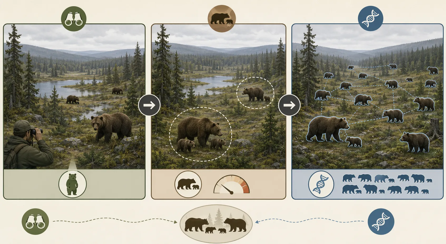
For a test passage, that Swedish result is the cleanest warning label. The female-with-cub count did not prove that bears were rare in the study area. It proved that this observation rule detected only a narrow, visible slice of the population. A count of observed animals is a measurement of encounters, not automatically a measurement of abundance.
The six methods below are best read as six different answers to the same detection problem. Each one decides what counts as a mark, how missed animals are handled, and which assumption has to survive field conditions.
| Method | What is sampled | How imperfect detection is handled | Best safe conclusion |
|---|---|---|---|
| Physical capture-mark-recapture | Captured and physically marked bears | Recapture histories estimate the fraction of marked animals missed later | Abundance can be estimated if closure and equal-detection assumptions are defensible |
| Non-invasive genetic mark-recapture | Hair or scat DNA profiles | Repeated genetic detections identify individuals and estimate detection probability | Strong abundance estimates when sampling covers the population and genotyping is reliable |
| Aerial photographic mark-resight | Bears photographed and re-identified from natural features or temporary marks | Marked or identifiable animals are modeled against later sightings | Useful landscape-scale density estimates when sighting and spatial assumptions are explicit |
| Line-transect distance sampling | Bears observed along survey lines | Detection is modeled as a function of distance from the transect | Efficient estimates when animals on or near the line are detectable and distances are accurate |
| Spatial capture-recapture | Individual detections at known camera, hair, or sampling locations | Detection declines with distance from an individual activity center | Density estimates are strong when individuals can be identified and spatial coverage is adequate |
| Sign occupancy surveys | Tracks, scat, hair, rubs, or other bear sign at sites | Repeated site visits estimate probability that sign is missed | Good for distribution or occupancy; weaker for direct abundance unless tied to stronger assumptions |
Why the Swedish Comparison Matters
A field count can fail in two ways that matter on an exam. First, the animal may exist but never enter the sampled area during the survey. Second, the animal may enter the sampled area but leave no usable detection. Female-with-cub counts add another filter: they observe only adult females currently accompanied by cubs, then infer from that visible class to the larger population. If reproduction, visibility, movement, observer effort, or sex-age structure varies, the inference can bend badly.
Mark-recapture logic is different. It does not pretend every bear is visible. It asks how often already known individuals are found again. If many known bears disappear from later samples, the model treats that as evidence of low detection, not as evidence that those bears stopped existing. That is the missing step in many weak ecology passages: the correction from observed individuals to estimated population.
The Swedish comparison also keeps cost in the frame without letting cost do the whole argument. Genetic sampling was cheaper than helicopter capture-mark-recapture in that evaluation, but the stronger scientific point was not simply that DNA saved money. It was that individual genetic identities let researchers estimate detection and abundance without physically handling every bear.[1]
Physical Capture-Mark-Recapture: Clear Logic, Heavy Field Cost
In the classic version, biologists capture bears, mark or collar them, release them, and then sample again. The marked-to-unmarked ratio in later samples helps estimate how many animals were present but not captured. The mark is literal: an ear tag, collar, tattoo, or other individual identifier.
The appeal is that the study design is easy to diagram. First sample: mark known individuals. Later sample: count how many marked animals return. If the second sample contains many unmarked animals and few marked ones, the model infers a larger population. If marked animals are commonly detected again, the population estimate is smaller.
The weak point is not the algebra; it is the assumption list. The population may need to be closed to births, deaths, immigration, and emigration during the sampling window. Marks must not be lost. Marked animals should not become much easier or harder to recapture because they were handled. Individuals with large home ranges, trap-shy behavior, or different habitat use can violate the equal-detection idea.
For brown bears, the practical burden is substantial. Helicopters, immobilization, trained crews, animal-welfare review, weather delays, and remote terrain all sit between a clean model and a real estimate. That is why non-invasive substitutions matter: they preserve the individual-identification logic while reducing the need to put hands on bears.
Evidence strength: strong as a statistical design when assumptions are met, but costly and intrusive for large, low-density bear populations. In the Swedish comparison, helicopter capture-mark-recapture provided the benchmark estimate of about 223 bears, while the simpler female-with-cub count badly undercounted the same population.[1]
Non-Invasive Genetic Mark-Recapture: Hair, Scat, and the Cleaner Inference
Genetic mark-recapture changes the mark from a collar to a DNA profile. Field crews collect hair from snag wires, scat from trails, or other biological material. A laboratory assigns samples to individuals when DNA quality allows. The same bear detected at multiple places or times becomes a recapture without ever being trapped.
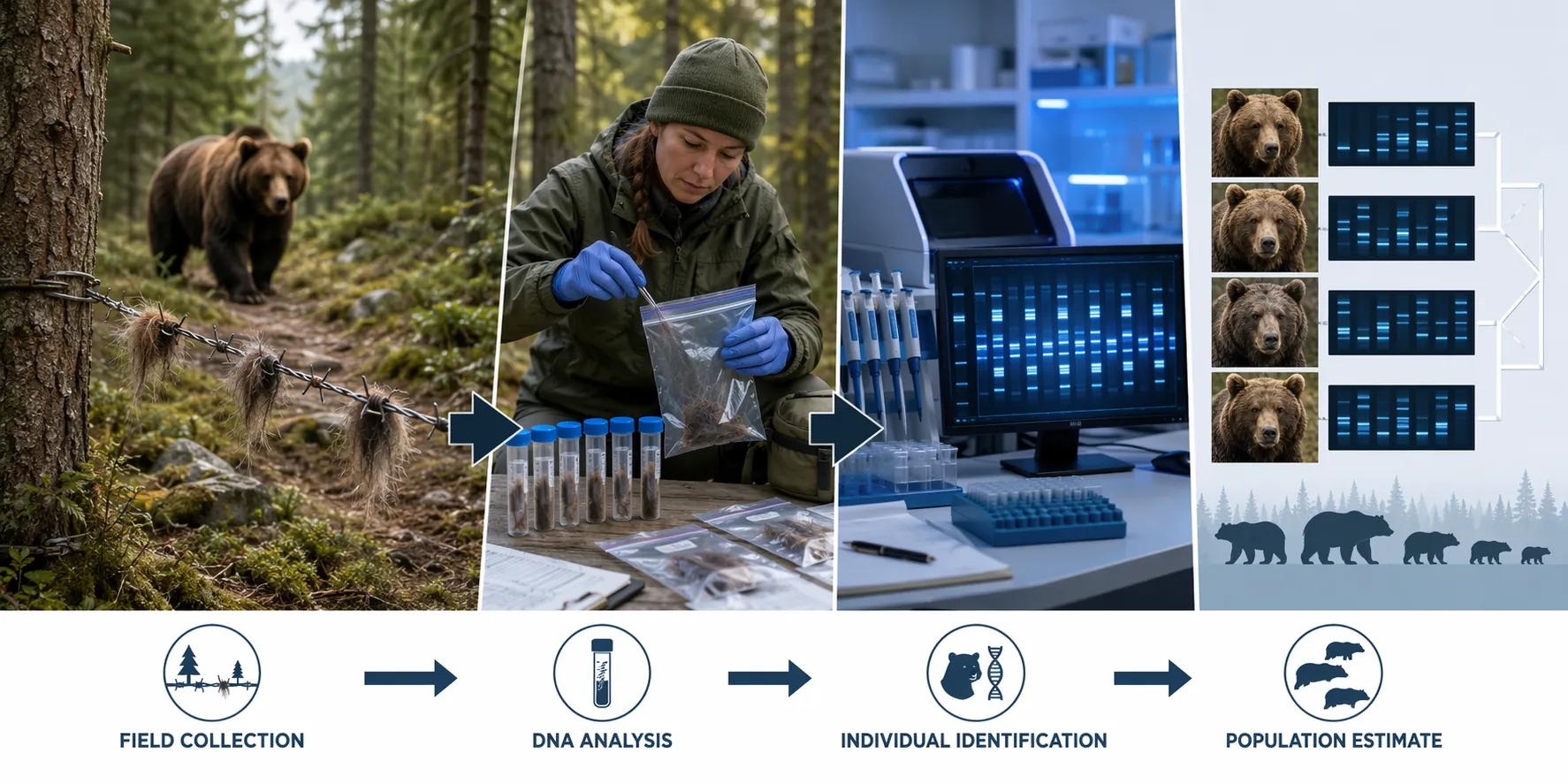
The core measurement is still a capture history. Bear A appears in week one and week three. Bear B appears once. Bear C appears at two different hair stations. The model uses those repeated and missed detections to estimate how many individuals were probably present but never sampled.
This method earns trust because it separates two questions that students often collapse. How many unique bears did the study identify? How many bears likely existed after correcting for detection probability? The first number is a minimum detected count. The second is an abundance estimate. In the Swedish evaluation, non-invasive genetic methods were rated most reliable and were far less expensive than helicopter-based capture-mark-recapture.[1]
A related Alaskan non-invasive monitoring example shows the same practical reason biologists use these designs. In a 19,998 km2 study area, Schmidt and colleagues estimated 420 independent bears with a 95% credible interval of 274 to 650 using a non-invasive mark-resight approach across a low-density landscape.[2] The wide interval is not a defect to hide. It tells the reader that detection was uncertain and that the estimate carries that uncertainty forward.
The break points are concrete. DNA can fail. Hair or scat may be unevenly distributed. Some bears may avoid sampling stations. Roads, rivers, berry patches, salmon streams, or human access can make some parts of the study area easier to sample than others. If the sampling grid misses an entire habitat type, the model cannot magically recover the bears that had almost no chance of entering the data.
Evidence strength: very strong for abundance when individual genotypes are reliable, spatial coverage is defensible, and detection probability is modeled rather than assumed away. For test purposes, this is one of the safest methods to recognize as an explicit correction for incomplete detection.
Aerial Photographic Mark-Resight: Less Handling, Still Not a Raw Count
Aerial photographic mark-resight surveys use aircraft and images rather than physical recapture. Bears may be identified or re-identified from photographs, natural features, collars, or temporary visual marks, depending on the design. The important shift is that a later sighting is treated as data about detection, not merely as another animal on a tally sheet.
A 2023 brown bear study found that non-invasive mark-resight surveys incorporating spatial information could reduce survey costs by 20% to 30%, corresponding to $40,000 to $60,000 in savings per survey, with little bias or precision loss in the evaluated setting.[3] In one cost-efficiency analysis, removing 51 subunits with elevation below 132 m reduced sampling effort by 27% while producing nearly identical density estimates: 40.6 versus 41.7 bears per 1,000 km2, with coefficient of variation changing from 17% to 20%.[3]
That result is useful because it shows what a defensible shortcut looks like. The study did not simply fly less and declare the count equivalent. It compared density estimates and precision after removing a defined part of the sampling frame. The consequence was measured: similar point estimates, modest precision loss, lower effort.
The assumption that can break this method is unequal visibility. Bears in open alpine terrain, river corridors, or low vegetation may be easier to photograph than bears under forest canopy. Weather and animal movement can also affect who is available to be seen. Spatial modeling helps, but it does not turn poor sighting conditions into complete detection.
Evidence strength: moderate to strong when spatial information, resighting probability, and survey design are explicit. It is especially useful where managers need broad-scale monitoring but cannot justify repeated physical capture.
Line-Transect Distance Sampling: Where the Bear Was Seen Matters
Line-transect distance sampling starts with a survey path. Observers travel along lines and record detected animals plus their perpendicular distance from the transect. The model expects detection to be highest near the line and lower farther away. Instead of asking only how many bears were seen, it asks how detection falls off with distance.
In Alaska, Becker and Quang's distance-sampling approach was reported as producing estimates that closely agreed with mark-recapture at much lower cost. A 2007 Alaska Department of Fish and Game article described a 21,035 km2 survey costing about $160,000, compared with several million dollars for genetic mark-recapture.[4] Those cost figures are useful as an agency-era comparison, not as current universal prices.
The exam-relevant assumption is sharp: animals on or very near the line must be detected with high probability, and distances must be measured accurately. If bears flee before detection, hide in cover, cluster near certain habitat features, or are missed even close to the transect, the detection curve can understate the population.
Evidence strength: moderate to strong in settings where aircraft or ground surveys can cover representative transects and detectability declines predictably with distance. It can be efficient, but it depends heavily on visibility, survey geometry, and observer performance.
Spatial Capture-Recapture: Detection Becomes a Map
Spatial capture-recapture, often shortened to SCR, adds location to individual detection histories. A bear detected at several camera stations, hair snares, or sampling points is not just counted as Bear A. Its detections are tied to places. The model estimates an activity center and uses the decline in detection with distance from that center to estimate density.
That spatial step matters because brown bears do not use a study area as evenly mixed particles. Some individuals live near the edge of the sampling grid. Some range widely. Some have activity centers close to traps or cameras; others have activity centers between them. SCR models make that geometry part of the abundance estimate rather than treating all individuals as equally available.
A major methods review identified SCR as a current gold standard for density estimation, while emphasizing that it requires individually identifiable detections.[5] The same review focused on low-density Asian bear species - sun, sloth, and Asiatic black bears - rather than brown bears, so its taxonomic scope should not be blurred. Its methodological lesson is still relevant: unmarked camera-trap methods often lack enough precision to detect even large declines of 80% to 90%.[5]
For brown bears, SCR can be built from genetic samples if DNA identifies individuals, or from images if individuals are visually identifiable. The second condition is harder for species without stable, unique pelage patterns. A camera trap that photographs an unmarked brown bear walking past may confirm presence, but it may not identify which bear it was. Without individual identity, the method becomes less powerful for abundance.
Evidence strength: very strong for density when individuals are identifiable and detector spacing matches movement scale. The common failure is not statistical sophistication; it is pretending that unmarked detections can answer the same question as individual capture histories.
Robust Capture-Recapture in the Pyrenees: Even Intensive Monitoring Misses Bears
The recovering Pyrenees brown bear population gives a useful correction to a tempting assumption: intensive monitoring does not equal complete detection. Vanpe and colleagues used Pollock's closed robust design to estimate abundance in a transboundary population that grew fivefold from 2008 to 2020, from 13 to 66 individuals.[6]
The striking part is that the model-based estimates were consistently lower than minimum-count figures.[6] That can feel backward if a student expects modeling always to inflate a count. The safer lesson is more precise: capture-recapture models estimate abundance under explicit detection and closure assumptions, while minimum counts summarize confirmed individuals. Depending on sampling structure and model assumptions, those quantities do not have to move in the same direction.
The Pyrenees case also changes how a reader should treat charismatic-population monitoring stories. A small, closely watched population can still contain detection gaps. Cross-border movement, uneven effort, and individual differences in detectability can matter even when managers and field teams are highly motivated.
Evidence strength: strong for showing why explicit capture-recapture modeling remains useful even in intensively monitored populations. The safe conclusion is not that minimum counts are useless; it is that they answer a narrower question than abundance models.
Sign Occupancy Surveys: Good Presence Data, Cautious Abundance Claims
Sign surveys look for indirect evidence: tracks, scat, hair, rub trees, feeding sign, or other traces. In occupancy designs, sites are visited repeatedly so the model can estimate two probabilities: whether the species uses a site and whether observers detect sign when it is present.
This is often the right tool when the question is distribution, range change, or broad monitoring across a large landscape. It is less direct when the question is population size. More sign does not automatically mean more bears, because sign production and detection can vary with movement, substrate, season, food availability, rainfall, observer effort, and trail placement.
The National Park Service describes sign occupancy alongside non-invasive mark-resight as a way to monitor low-density brown bear populations across large landscapes, including the Alaskan work that estimated 420 independent bears with a 95% credible interval of 274 to 650.[2] The pairing is important: sign can extend spatial monitoring, while individual-based methods carry more of the abundance inference.
Evidence strength: useful for occupancy and distribution; weaker for direct abundance unless combined with models or auxiliary data that connect sign detection to animal numbers. On an exam, treat sign occupancy as a detection-corrected presence method before treating it as a population-size method.
How to Judge a Brown Bear Population Ecology Study
When a passage describes a brown bear population ecology study, look for the point where observation becomes inference. The method may involve vials of hair, scat bags, flight lines, photographs, collars, camera stations, or muddy tracks. The reasoning test is the same.
- What is sampled: individuals, DNA profiles, photographs, transect sightings, detector locations, or sign at sites.
- What is missed: animals outside the sampled area, animals present but unseen, samples that fail genotyping, photographs that cannot identify individuals, or sign that observers fail to detect.
- What correction is used: recapture probability, resighting probability, distance-based detection, spatial detection around activity centers, or occupancy detection probability.
- Which assumption can break it: closure, equal detectability, mark retention, representative transects, individual identification, detector spacing, or stable site occupancy.
- What conclusion is safe: abundance, density, distribution, trend, or only a minimum confirmed count.
The strongest designs for abundance are usually the ones that identify individuals and model detection explicitly. Genetic mark-recapture and SCR stand out because they can turn repeated detections and missed detections into an estimate with uncertainty. Physical capture-mark-recapture has the same inferential backbone but carries higher cost and welfare burdens. Aerial mark-resight and distance sampling can be efficient when visibility and spatial assumptions are handled honestly. Sign occupancy is valuable, but it usually answers a less direct question.
The geographic caveat is real. Much of the brown bear methods literature used here is Alaskan or Scandinavian, with an additional methods review drawn from Asian bear species rather than brown bears specifically.[1][2][3][5] Dense forest, open tundra, mountain terrain, road access, political borders, and laboratory capacity can change which method is realistic. A trustworthy estimate is not the fanciest model on paper. It is the design whose sampling frame, detection model, budget, animal-welfare constraints, and precision needs match the population being studied.
References
- An evaluation of field and non-invasive genetic methods to estimate brown bear (Ursus arctos) population size - ScienceDirect, 2006.
- Using non-invasive mark-resight and sign occupancy surveys to monitor low-density brown bear populations across large landscapes - National Park Service.
- Non-invasive mark-resight surveys for brown bears: Incorporating spatial information to improve landscape-scale monitoring of density and distribution - Wiley Online Library, 2023.
- Better Tools for Counting Bears - Alaska Department of Fish and Game, 2007.
- Comparison of methods for estimating density and population trends for low-density Asian bears - ScienceDirect, 2022.
- Estimating abundance of a recovering transboundary brown bear population with capture-recapture models - Peer Community Journal, 2022.
Comments
Join the discussion with an anonymous comment.