
SAT Exam Hub
How to Study the Analog AI Patent Landscape
Learn a systematic six-step method for patent landscape analysis, using the analog AI (in-memory computing) field as a real-world case study. Understand how to scope, search, analyze, and visualize patent data for any technology area.
- SAT
- ACT
- GRE
- MCAT
- ASVAB
- digital-sat
- adaptive-testing
- registration-fee
- content-outline
- score-target
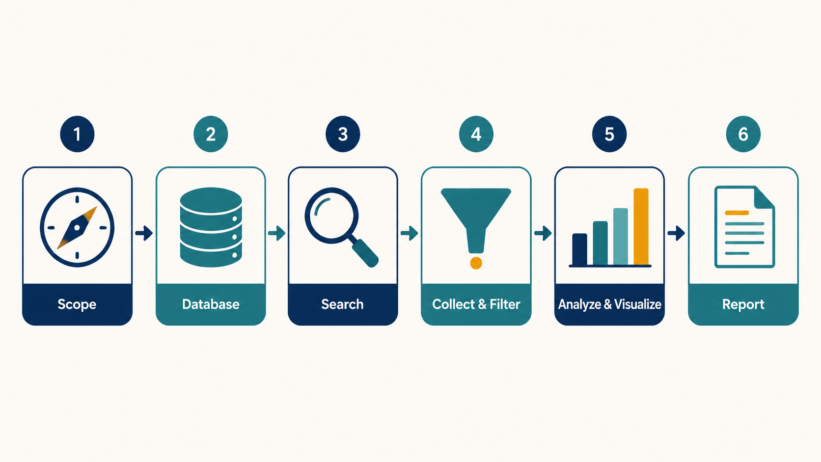
Studying a patent landscape is mostly an exercise in boundary setting. With about 3.7 million global patent filings in 2024, the problem is not whether there is enough material, but how to turn a sprawling technology phrase into a search scope another analyst can reproduce. WIPO's landscape guidance and practitioner guides from IamIP and Patsnap all converge on the same six-step loop: scope, choose databases, search, collect and filter, analyze and visualize, then report. [1][2][3]
Analog AI is a useful worked example because the field is easy to oversell. IBM, Mythic, and Quanta all describe energy-efficiency gains that are often framed as more than 1,000x versus digital AI chips, but that is a technology claim, not a patent-landscape conclusion. [7][8][9] For the analyst, the real value is that the field is current, contested, and messy enough to show why scope discipline matters.
Start With Scope, Not Keywords
The first trap is treating analog AI as a keyword instead of a boundary. For a usable study, decide whether the topic means in-memory analog computing, the broader neuromorphic umbrella, or both; decide whether device substrates, circuit techniques, and application domains will sit in one bucket or in separate ones; and write those choices down before you run the search. That is what makes the study reproducible for the next person, not just persuasive for you.
- Count patent families or publications, because those two views answer different questions.
- Fix the jurisdictions and date window before the first query, then keep them unchanged through the first pass.
- Separate the substrate from the application, so a memory technology is not accidentally counted as a use case.
- Write exclusion rules for broad terms like neuromorphic, because scope drift usually starts there.
If you use this method to study a syllabus rather than a technology field, the same habit shows up in How to Create a Study Guide from Your Syllabus in 5 Steps: define the boundary first, then gather evidence inside it.
The Six-Step Workflow Is Not One Pass
| Step | What it decides | What usually goes wrong |
|---|---|---|
| 1. Scope | What counts as the technology and what stays out | Starting with a keyword list before the research question is fixed |
| 2. Database selection | Which patent sources will be searched | Assuming one platform is enough for a global view |
| 3. Search construction | How concepts, synonyms, and exclusions are translated into queries | Mixing device names, applications, and buzzwords in the same string |
| 4. Collection and filtering | How families, duplicates, and borderline hits are handled | Letting database labels stand in for human review |
| 5. Analysis and visualization | Which clusters, trends, and comparisons are actually defensible | Treating every chart as a conclusion instead of a filter on the data |
| 6. Reporting | What the reader can safely infer and what remains uncertain | Turning counts into market certainty |
That loop is intentionally iterative. A first search usually sends you back to the scope, because the point of the method is not to finish quickly but to make the final boundary explicit enough that someone else could rerun it.
What the Analog AI Search Actually Surfaces
IAM Media reported 5,913 analog AI patent families from 2015 to 2025 across USPTO, EPO, WIPO, CNIPA, and KIPO. Because that source sits behind a paywall, the count works best as a second-hand benchmark rather than as a primary dataset you can audit line by line. Even so, it is a useful working number: large enough to show real clustering, but still small enough to keep the analysis legible. [4]

Patsnap's in-memory analog computing landscape organizes the field into four NVM technology clusters and four innovation phases. Those categories are not the only way to slice the data, but they are useful because they make the landscape analyzable without pretending the field is cleaner than it is. [5]
| Technology cluster | Why it matters |
|---|---|
| RRAM crossbar arrays | The most visible compute-in-memory hardware path in the landscape [5] |
| Flash-based analog neural memory | Shows how mature storage platforms are reused for analog AI [5] |
| Memcomputing / logic-in-memory | Captures work that emphasizes computation inside the storage fabric [5] |
| NV-TCAM / CAM for AI search | Connects analog ideas to matching and search workloads [5] |
The phase view runs from instrumentation roots (1980 to 1995), to the memcomputing paradigm (2014 to 2016), to RRAM consolidation (2019 to 2021), and then to system-level integration (2022 to 2025). The point of that timeline is not nostalgia; it shows that current filings sit on older ideas about memory, measurement, and control rather than appearing from nowhere. [5]
Use Neuromorphic as a Boundary Check
If you widen the net to neuromorphic computing, Patsnap's 2026 landscape counts 7,478 families, with NVIDIA at 679, IBM at 632, and Samsung at 564 among the top assignees. The same source says the category peaked at 1,134 families in 2021 and fell to 699 in 2024. That does not make neuromorphic the same as analog AI; it makes it a useful contrast case, because overlap is exactly where scope drift tends to hide. [6]
For this study guide, that contrast matters. If the question is in-memory analog computing, a broader neuromorphic bucket belongs in a comparison chart or appendix, not in the core dataset.
Report Boundaries, Not Hype
- Say whether the count is by family, publication, or jurisdictional filing, because the same invention can look larger or smaller depending on the unit.
- Label second-hand figures as benchmarks when the source is behind a paywall or otherwise not directly auditable.
- Keep substrate claims separate from market claims, since a patent map can show activity without proving commercial leadership.
- State exclusions plainly, especially where non-English filings, older families, or adjacent technologies may be undercounted.
That is also where litigation-cost context belongs, if you use it at all. IamIP cites average patent litigation costs of $2.3 million to $4 million per case and says 95% to 97% of disputes settle when the IP terrain is mapped, which is enough to explain why landscape work gets funded, but not enough to turn the article into an IP risk memo. [2]
A good landscape report leaves the reader with a defensible shape, a clear method, and enough uncertainty flags to avoid pretending the count is the conclusion. Analog AI is a strong teaching case because it is large, current, and fragmented enough to show how the method works without requiring deep prior-art expertise.
References
- WIPO Guidelines for Preparing Patent Landscape Reports. WIPO
- How to do a patent landscape analysis: step-by-step guide. IamIP
- Patent landscape analysis guide 2025. Patsnap
- Analog AI: The IP landscape ahead of the market. IAM Media. July 21, 2026
- In-memory analog computing landscape 2026. Patsnap
- Neuromorphic Computing Patent Landscape 2026. Patsnap
- Analog AI. IBM Research
- Analog Computing. Mythic AI
- What Is Analog Computing?. Quanta Magazine. August 2, 2024
Related exhibits & inventory
Verified outcomes
No verified outcomes on file for this exam yet
See Methodology for how outcome evidence is disclosed once logged.
Planners
No planner filed for this exam yet
A downloadable timeline template for this exam hasn't been published yet.
Tool verdicts
AI-tool cautions
No AI tools tested for this exam yet
No hands-on AI-accuracy logs have been filed for this exam.
Questions about this plan
Ask a question about a specific section, timeline, or citation in this plan — or flag something that needs correcting.
Comments
Join the discussion with an anonymous comment.